The F-statistic you see in OLS output
Some time ago, I gave a derivation for the t-test in standard OLS output (link) , and how to compute a confidence ellipse for all parameters jointly in the linear model. I did not give the derivation of the F-statistic reported in the OLS regression summary output. I will do that in this post.
Consider a linear model \(Y = X_{N}\beta _N + e\) where \(e \sim \mathcal N(0,\sigma^2 I_n)\) . This is our null hypothesis. Subscript \(N\) is for “null”. \(X_N\) is a design matrix, i.e. each row of \(X_N\) is a sample, and each column is one of the \(p\) covariates.
We are curious whether some other covariates \(X_{E}\) might be relevant. This is the alternative hypothesis, namely that the data generator is instead
\[Y = X_{N}\beta _N + X_{E}\beta _E + e\]where \(e \sim \mathcal N(0,\sigma^2 I_n)\) like before. The null hypothesis would be that \(\beta_E = 0\), and we want to test against the alternative that \(\beta_E \neq 0\). Subscript \(E\) is for “extra”. We will call the regression model for the alternative hypothesis the “unrestriced model” and under the null hypothesis we call it the “null model”.
The full design matrix of the alternative hypothesis is \(X^T_A = [X_N^T, X_E^T]\). Assume that this matrix has full rank, i.e. \(\rank{X_A} = p+s\), where \(s\) is the number of extra covariates in \(X_E\).
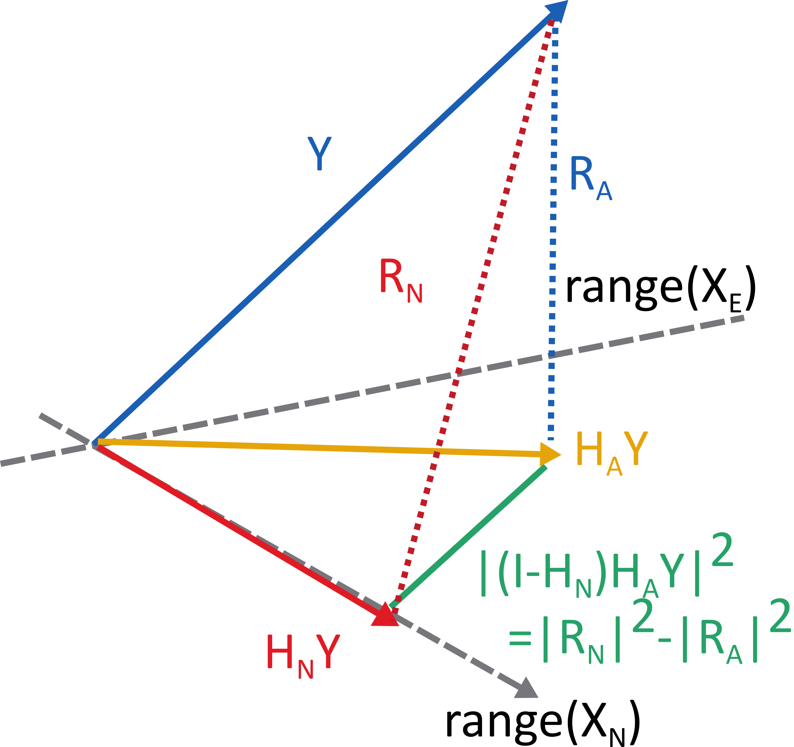
The residuals from the regression of the null model is \(R_N = Y - X_N\hat\beta_N\). This is \(R_N = (I - X_N(X_N^TX_N)^{-1}X_N^T)Y\) by standard OLS. By the hat matrix of the null model \(H_N \coloneqq X_N(X_N^TX_N)^{-1}X_N^T,\) we rewrite the residuals as \(R_N = (I-H_N)Y\).
One can also project onto the alternative model as well to get the alternative residuals, \(R_A = (I-H_A)Y\), where \(H_A = X_A(X_A^TX_A)^{-1}X_A^T\).
Next key observation is that the range of \(H_A\) is the linear space spanned by the range of \(H_N\) and \(H_E\). So one can first project \(Y\) onto the alternative with \(H_A\), and then take the residual of that, when projecting onto the range of \(X_N\). This residual, lets call it \(\tilde{R}\), has the norm \(\norm{\tilde{R}}^2 = \norm{(\eye - H_N)H_AY}^2 = \norm{R_N}^2 - \norm{R_A}^2\), where the second expression follows from the geometry.

We know, \(R_A = (\eye{} - H_A)Y\), with \(H_A\) having rank \(p+s\) so \(\norm{R_A}^2/\sigma^2 \sim \chi^2_{n-p-s}\). This is just like we treated the residuals in the previous blog post.
Algebra shows \(\tilde{R} = (\eye{} - H_N)H_AY = (\eye{} - H_N)X_E\beta_E + (\eye{}-H_N)H_Ae\). The first term is zero under the null hypothesis. The second term is rank-\(s\)-projection of a gaussian so \(\frac{\norm{R_N}^2 - \norm{R_A}^2}{\sigma^2} = \norm{\tilde{R}}^2/\sigma^2 \sim \chi^2_{s}\) by the same logic as before.
The two residuals, \(R_A\) and \(\tilde{R}\) are uncorrelated, since they are projections onto orthogonal subspaces. Since they are gaussian this also means they are independent. So the quotient of their norms is \(F\) distributed with \(s\) and \(n-p-s\) degrees of freedom.
\[F = \frac{\norm{\tilde{R}}^2 / \sigma^2}{s} \cdot \frac{n-p-s}{ \norm{R_A}^2/\sigma^2 } = \frac{(\norm{R_{N}}^2 -\norm{R_A}^2)/s}{\norm{R_A}^2/(n-p-s)}\]In many texts, they use the notation for residual sum of squares, and write
\[F = \frac{(RSS_{N} - RSS_{A})/s}{RSS_A/(n-p-s)}\]Three applications
If \(X_N\) is the column vector of ones (\(p=1\)), and \(X_E\) is all other covariates, the \(F\)-statistic so computed is the one reported in the OLS output. Deriving this test statistic was the purpose of this post.
Another application is when \(X_E\) is the interaction between features in \(X_N\) and some binary group indicator (being \(0\) or \(1\)). Some observations are then explained by \(\beta_N\), and the other get regression coefficients \(\beta_N + \beta_E\). The null hypothesis is that \(\beta_E = 0\), i.e. not difference in regression coefficients between the groups. This is often called a Chow test after a influential test for equality of regressions. 1.
Testing for equality of regression functions between groupss has also been employed in Invariant Causal Prediction (ICP) 2, which has connection to my research field.
Comments on the assumpation
Under the alternative, we expect a bias term in the numerator, and the \(F\)-statistic will be larger than under the null. Therefore, do a onesided test in \(F\).
We needed to assume homoscedacity. This may be dealt with. See e.g. 3.
We needed to assume the true data generator was a linear gaussian model. This is quite strong. To relax this assumption, other techniques must be employed.
-
Chow, G. C. (1960). Tests of equality between sets of coefficients in two linear regressions. Econometrica: Journal of the Econometric Society, 591-605. https://www.jstor.org/stable/1910133 ↩
-
Schmidt, Peter, and Robin Sickles. “Some further evidence on the use of the Chow test under heteroskedasticity.” Econometrica: Journal of the Econometric Society (1977): 1293-1298 https://www.jstor.org/stable/1914076 ↩
-
Peters, J., Bühlmann, P., & Meinshausen, N. (2016). Causal inference by using invariant prediction: identification and confidence intervals. Journal of the Royal Statistical Society Series B: Statistical Methodology, 78(5), 947-1012. https://doi.org/10.1111/rssb.12167 ↩
