
Classical OLS
I have several times seen various ways to motivate the ordinary least squares regression. Even Wikipedia have several ways to motivate/derive it. However, most motivations are filled with statistical – rather than mathematical – jargon, and can be difficult to track. So this post aims at motivating the classical OLS, the F-statistic found in the output of many libraries such as statsmodel and so on. Here goes.
We use \(\E\) to denote expectation. The notation \(\E_n\) is the empirical expectation, i.e. average over \(n\) iid datapoints \(\E_n[q] = \frac{1}{n}\sum_{i=1}^{n}q_i\), where \(q_i\) are iid observations distributed by the distribution \(P_q\). The empirical expectation is in turn a new random variable.
Classical Gaussian OLS
More or less a copy of the derivation on CV.SE
Given a fixed, nonrandom design matrix \(X \in \R^{n\times d}\), whose columns are \(n\) observations and rows are \(d\) features, and outcome vector \(y\). Assume that \(y = X\beta _\circ + e\) where \(e \sim \mathcal N(0,\sigma^2 I_n)\) i.e. gaussianity, homoscedacity
Point estimate
Least squares estimation for the parameter vector \(\beta\) is solving the equation \(\argmin_\beta |y-X\beta |^2\) and it is solved by \(\hat \beta = (X^TX)^{-1} X^Ty\)
Some algebra shows \(\hat \beta = \betaTrue + (X^TX)^{-1} X^Te\), and that implies \(\hat \beta \sim \mathcal N ( \betaTrue, (X^TX)^{-1} X^T \sigma^2 X (X^TX)^{-1}) = \mathcal N ( \betaTrue, (X^TX)^{-1}\sigma^2)\) which implies that we have a standard normal pivot quantity \begin{equation} z\coloneqq \frac{(X^TX)^{1/2}}{\sigma} \left( \hat \beta -\betaTrue \right) \sim \mathcal N ( 0, \eye_d) \label{eq:classical:z} \end{equation}
If the residual noise standard deviation \(\sigma\) was known, we could say something about the distribution of the estimate.
Estimating the noise
We will now estimate \(\sigma\) from the data instead, and see where that takes us. Maybe it can give us some other useful distribution, albeit not as nice as the simple standard normal.
Define the fit residuals \(\hat e = y-\hat y = y - X \hat \beta\) and the annihilator matrix \(M = \eye_n - X (X^TX)^{-1} X^T\) so that \(\hat e = My\) Note that \(M^2=M\), a property called idempotence. It is a projection matrices, and projects onto the nullspace of \(X\). For such a matrix, their rank is easy to compute, since it coincides with its trace. (all eigenvalues are \(0\) or \(1\)).
\[\begin{align} \rank{M} & = \trace{M} \\ & = \trace{\eye_n} - \trace{X (X^TX)^{-1} X^T} \\ & = n - \trace{\eye_d} \\ & = n-d \end{align}\]Define the estimator \(s^2\) and apply some algebra. We utilize \(M^T=M\) and \(MX=0\).
\[\begin{align} s^2 & = \frac{1}{n-d} \|\hat e \|^2 \\ & = \frac{1}{n-d} y^TM^TMy \\ & = \frac{1}{n-d} (X\hat \beta + e) ^TM(X\hat \beta + e) \\ & = \frac{1}{n-d} e^TMe \\ \end{align}\]Breaking things a little \(\frac{n-d}{\sigma^2}s^2 = \frac{e}{\sigma}^TM\frac{e}{\sigma} \eqqcolon V\) and applying Theorem 2 from Styan1 , to obtain that \(V \sim \chi^2_{n-d}\).
Notice that this step used the crucial assumption of normality in the residuals.
We now obtained a new pivotal quantity, involving the unknown noise variance \(\sigma^2\). Can somehow cancel the unknown things from the two pivots?
Getting the Confidence Intervals
Notice that \(\hat \beta\) is normally distributed. So is also \(\hat e = M e\). They are also uncorrelated since \(M\) projects onto the nullspace of \(X\), and \(\hat \beta\) lies in the row space of \(X\). Uncorrelated gaussians are independent, which is proven in many probability courses. See e.g. Theorem 7.1, Chapter 5, in the book of Gut. 2
The idea we will follow, which exploits this fact, is that the joint PDF will factorize, since the precision matrix will have a block form. We have \(V\), which is a function of \(\hat e\), so it is also independent from \(\hat \beta\). The pivot \(z\) is a function of \(\hat \beta\) so it must be independent from \(V\).
It seems we will get our cancellation!
Confidence for a single parameter, confidence box
Let \(z_k\) denote the \(k\)th component of \(z\) from before. It will be distributed \(z_k \sim \mathcal{N}(0,1)\), and \(V \sim \chi^2_{n-d}\) then \(t_k \coloneqq \frac{z_k}{\sqrt{V / (n-d)}} \sim t_{n-d}(0,\eye_d)\) follows a Student \(t\) distribution.
We can also write \(z_k = \frac{1}{\sigma \sqrt{S_{kk}}} \left( \hat \beta_k -\beta_{\circ k} \right)\) where \(S_{kk}\) is the \(k\)th diagonal of \((X^TX)^{-1}\).
\[\begin{align} t_k & = \frac{z_k}{\sqrt{V / (n-d)}} \\ & = \frac{\frac{1}{\sigma \sqrt{S_{kk}}} \left( \hat \beta_k -\beta_{\circ k} \right)}{\sqrt{\frac{\frac{n-d}{\sigma^2}s^2}{n-d}}} \\ & = \frac{\left( \hat \beta_k -\beta_{\circ k} \right)}{\sqrt{ s^2S_{kk}}} \\ & = \frac{ \hat \beta_k -\beta_{\circ k} }{\hat{se}(\hat \beta)} \label{eq:ols:standard result} \end{align}\]where \(\hat{se}(\hat \beta) \coloneqq \sqrt{ s^2S_{kk}}\) is the estimated standard error of the estimator. This presentation is probably the most standard presentation of the \(t\) statistic in linear regression.
This t-statistic can be used in hypothesis test for a single coefficient being zero, or inverted to form a confidence interval. When there are multiple coeffients, these intervals generalize to a confidence box. The box may be adjusted via bonferroni adjustment, but these will form correlated hypothesis tests, so the confidence box is an approximation only.
Confidence ellipse
Since the different \(t\)-statistics are dependent, we must do some higher dimensional generalization of the argument above.
Moreover, \(\norm{z}^2 \sim \chi^2_{d}\), so we can get a test statistic that is Snedcor \(F\)-distributed. \(\frac{\norm{z}^2/d}{V/(n-d)} \sim F(d,n-d)\) Let \(\tau_\confLevel = F^{-1}_{1-\confLevel}(d,n-d)\) be the inverse cdf at \(1-\alpha\) for the F-distribution. Then
\[\begin{align} \Pr \left[ \frac{\norm{z}^2/d}{V/(n-d)} \leq \tau_\confLevel\right] &= 1-\confLevel \\ \Pr \left[ \frac{\norm{(X^TX)^{1/2}(\hat\beta - \betaTrue)}^2/d\sigma^2}{s^2/\sigma^2} \leq \tau_\confLevel\right] &= 1-\confLevel \\ \Pr \left[ (\hat\beta - \betaTrue)^{T} \frac{X^TX}{ds^2\tau_\confLevel}(\hat\beta - \betaTrue) \leq 1\right] &= 1-\confLevel \end{align}\]Intermezzo: quadratic forms
Assume you have a positive definite matrix \(Q\), with eigenvalues \(\lambda_i\) and eigenvectors \(v_i\). The equation \(x^{T}Qx \leq 1\) represents a ellipsoid where the \(i\)th semiaxis has direction \(v_i\) and length \(1/\sqrt{\lambda_i}\). Equivalently, the equation for the same ellipse may be written \(\norm{Q^{-1/2}x}\leq 1\). This is the form I utilize in the code to actually draw the ellipse.
The true parameter will with probability \(1-\confLevel\) lie in an ellipse centered at \(\hat \beta\) and with a shape determined by the eigenvectors and eigenvalues of \(\frac{X^TX}{ds^2\tau_\confLevel}\).
We can also comput the value \(\frac{\norm{z}^2/d}{V/(n-d)}\) to obtain a test-statistic used for hypotheis testing.
Illustration of the results
The following illustrates a classical OLS regression. It generates some data from \(y=0.5+0.2x\) with standard normal \(x\). Then is runs a well specifed regression using statsmodels.
OLS Regression Results
==============================================================================
Dep. Variable:                      y   R-squared:                       0.059
Model:                            OLS   Adj. R-squared:                  0.049
Method:                 Least Squares   F-statistic:                     6.128
Date:                Wed, 13 Oct 2021   Prob (F-statistic):             0.0150
Time:                        11:04:59   Log-Likelihood:                -106.30
No. Observations:                 100   AIC:                             216.6
Df Residuals:                      98   BIC:                             221.8
Df Model:                           1
Covariance Type:            nonrobust
==============================================================================
                coef    std err          t      P>|t|      [0.025      0.975]
------------------------------------------------------------------------------
const          0.5433      0.071      7.677      0.000       0.403       0.684
x              0.1673      0.068      2.476      0.015       0.033       0.301
==============================================================================
Omnibus:                        1.651   Durbin-Watson:                   2.049
Prob(Omnibus):                  0.438   Jarque-Bera (JB):                1.123
Skew:                          -0.104   Prob(JB):                        0.570
Kurtosis:                       3.475   Cond. No.                         1.05
==============================================================================
The std error is as described above, and it presents the t-statistic under the null hypothesis that a specific coefficient is zero, and the others being whatever they like. It also presents the F-statistic under the joint hypothesis of all the coefficients except the intercept being zero. The F-statistic in the statsmodels output is this different from the one I computed! Beware! This F-test is rather a maximum likliehood ratio test, as used in ANOVA for model fit comparisons. But that is a separate story and not part of this post.
UPDATE: I wrote about this later in this post.
The F-based confidence ellipse and box are presented in a plot below.
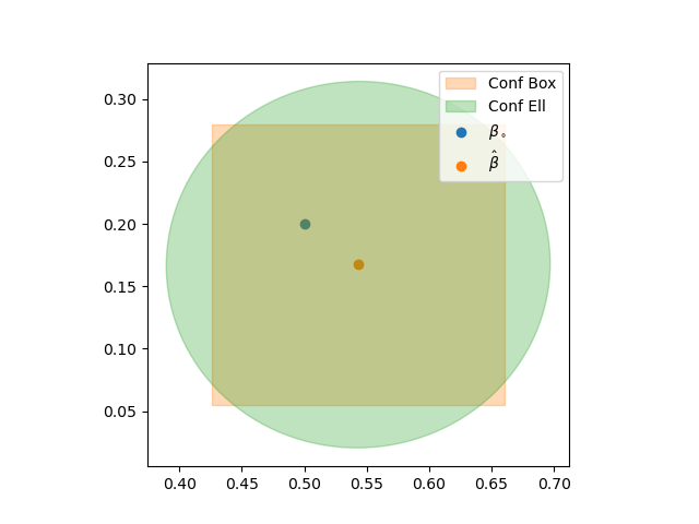
The code to produce the plot and the regression summary also includes manual calculation of some of the quantities, so it might be a nice reference computation. See below
-
G. P. H. Styan, Notes on the distribution of quadratic forms in singular normal variables, Biometrika, vol. 57, no. 3, pp. 567–572, 1970, doi: 10.1093/biomet/57.3.567. ↩
-
A. Gut, An Intermediate Course in Probability, 2nd ed. Dordrecht : New York, NY: Springer, 2009. ↩