Probability theory definitions by example

This post is a note-for-memory regarding definitions in probability theory, and how they relate, by giving a simple example.

The basic probability space

Define a set \(\mathbb 6 = \{A,B,C,D,E,F\}\) - a set of six elements. We use letters to name the elements but there is no structure a priori on \(\mathbb 6\) such as ordering. We will call this set a sample space, as is customary in probability. We will also use the notation \(\Omega = \mathbb 6\).

Lets now give the set some structure! Define the powerset \(\mathfrak P(\mathbb 6)\) - the set of all subsets of \(\mathbb 6\). This set is a \(\sigma\)-algebra, so we say that the tuple \((\mathbb 6,\mathfrak P(\mathbb 6))\) is a measurable space. The \(\sigma\)-algebra over the sample space is typically notated \(\mathcal F\), so we will stick to that too. In the context of probability, we will call the elements of the \(\sigma\)-algebra events, and in more general measure theory.

Further, define a function \(P : \mathcal F = \mathfrak P(\mathbb 6) \to \mathbb R\). By requiring countibly additivity, \(P(\bigcup_{k=1}^{\infty} A_k)= \sum_{k=1}^{\infty} P(A_k)\) for disjoint sets \(A_k\), and noting that it is enough to define the function over the singletons in the \(\sigma\)-algebra, the \(\{\omega\} \in \mathcal F\). They are called elementary events. In our example, they are the events \(\{\{A\},\{B\},\{C\},\{D\},\{E\},\{F\}\}\). Lets take \(P\) as per the table below.

\(A \in \mathcal F = \mathfrak P(\mathbb 6)\)	\(P(A)\)
\(\{A\}\)	\(1/8\)
\(\{B\}\)	\(3/8\)
\(\{C\}\)	\(1/8\)
\(\{D\}\)	\(1/8\)
\(\{E\}\)	\(1/8\)
\(\{F\}\)	\(1/8\)

We say that \(P\) is a measure, since \(P(A)\geq 0 \, \forall A\in \mathcal F\), and countable additivity. We call the triplet \((\Omega,\mathcal F, P)\) a measure space.

We can verify that \(P(\Omega)=1\) and therefore we call \(P\) a probability measure and \((\Omega,\mathcal F, P)\) a probability space or probability triplet.

Random elements

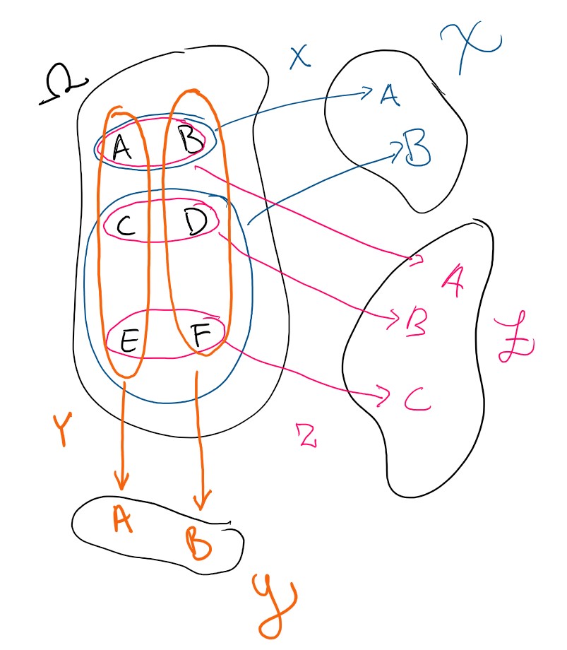
Start with defining the first random element - \(X\). It is a function from \(\Omega\) to \(\mathbb 2 = \{1,2\}\). Since \(\mathbb 2\) has a \(\sigma\)-algebra defined by the powerset \(\mathcal F_X = \mathfrak P(\mathbb 2)\), the tuple \((\mathbb 2,\mathfrak P(\mathbb 2))\) is also a measurable space. Introduce \(X\) like

\[X(k) = \begin{cases} 1 & \text{ if } k\in \{A,B\}\\ 2 & \text{ else} \end{cases}\]

One can verify that \(\forall A \in \mathfrak P(\mathbb 2)\) it holds that the inverse image of every event over \(\mathbb 2\) is an event over \(\Omega\):

\[X^{-1}(A)= \{ k \in \Omega | X(k)\in A\} \in \mathcal F\]

All functions that fulfil this criterion are called measurable. Since the definition relies on our choice of \(\sigma\)-algebra, we clarify this by saying that \(X: (\Omega,\mathcal F) \to (\mathbb 2,\mathfrak P(\mathbb 2))\) is measurable - it is a function between measurable spaces, not between sets. Let \(\mathcal X = \operatorname{ran}X\) denote the range of \(X\). In this case, the random element is surjective, so \(\mathcal X = \mathbb 2\). We can then restrict the codomain \(\sigma\)-algebra to the range, and get a new measurable space on which \(X\) is surjective, i.e. \(\mathcal F_X = \{ \mathcal X \cap A | A \in \mathfrak P(\mathbb 2)\}\).

\[X: (\Omega,\mathcal F) \to (\mathcal X,\mathcal F_X)\]

We will call \(X\) a \(\mathbb 2\)-valued random variable, or a random element, since it is a measurable function with a probability space as domain.

Without any qualifying words, the term random variable is reserved for measurable functions \((\Omega,\mathcal F) \to (\mathbb R,\mathcal R)\) specifically, where \((\Omega,\mathcal F,P)\) is a probability space, \(\mathbb R\) is the real numbers and \(\mathcal R\) is the Borel algebra. This example I develop in this post are not random variables, but about random elements.

We define the random element \(Y: (\Omega ,\mathcal F) \to (\mathbb 2,\mathfrak P(\mathbb 2))\) by \(Y(A)=Y(C)=Y(E)=A\) and \(Y(B)=Y(D)=Y(F)=B\). Define also the random element \(Z: (\Omega ,\mathcal F) \to (\mathbb 3,\mathfrak P(\mathbb 3))\) by \(Z(A)=Z(B)=A\) and \(Z(C)=Z(D)=B\) and \(Z(E)=Z(F)=C\). Introduce \((\mathcal Y, \mathcal F_Y)\) and \((\mathcal Z,\mathcal F_Z)\). as the ranges of the random variables, and the \(\sigma\)-algebras on those ranges.

Concept map with random elements. Notice that Z and Y 'project' out different axes of the set Omega, even though Omega has no structure in itself. You can also notice that Z has strictly better 'resolution' than X

Side note on continous functions

The criteria for measurable functions is completely analogous with the criteria of continous functions on topological spaces. Just like continous functions respect topology, measurable functions respect \(\sigma\)-algebras. I summarize it in the table below. You can notice that since Probability is “simply” measure theory on measure of total measure 1, they have partially the same jargon.

Topology	Measure Theory	Probability
Topology	\(\sigma\)-algebra	\(\sigma\)-algebra
Open sets	Measurable sets	Events
Topological space	Measurable space	Measurable space
n/a	Measure space	Probability space
n/a	Measure	Probability Measure
Continuous functions = The inverse image of open sets are open sets	Measurable functions = The inverse image of measurable sets are measurable sets	Measurable functions = The inverse image of events are events

Generated \(\sigma\)-algebras, measurability with respect to a random element, filtration

The probability space and random variables models phenomenon in the real world. Elements in the sample space \(\Omega\) are the the possible outcomes that could happen if we make an observation of a random system. However, these elements are not part of the \(\sigma\)-algebra, so we cannot say anything about their probabilites. But we have the elementary events in the \(\sigma\)-algebra, so we may work with them.

Lets use the following interpretation of our elementary events:

\(\{k\} \in \mathcal F = \mathfrak P(\mathbb 4)\)	Interpretation
\(\{A\}\)	Person is a tall smoker
\(\{B\}\)	Person is a tall non-smoker
\(\{C\}\)	Person is a normal height smoker
\(\{D\}\)	Person is a normal height non-smoker
\(\{E\}\)	Person is a short smoker
\(\{F\}\)	Person is a short height non-smoker

This also gives is interpretations of the elementary events in \(\mathcal F_X=\mathfrak P(\mathbb 2)\) , \(\mathcal F_Y=\mathfrak P(\mathbb 2)\) and \(\mathcal F_Y=\mathfrak P(\mathbb 3)\).

\(\{k\} \in \mathcal F_X = \mathfrak P(\mathbb 2)\)	Interpretation
\(\{A\}\)	Person is tall
\(\{B\}\)	Person is not tall

\(\{k\} \in \mathcal F_Y = \mathfrak P(\mathbb 2)\)	Interpretation
\(\{A\}\)	Person is a smoker
\(\{B\}\)	Person is a non-smoker

\(\{k\} \in \mathcal F_Z = \mathfrak P(\mathbb 3)\)	Interpretation
\(\{A\}\)	Person is tall
\(\{B\}\)	Person is normal height
\(\{C\}\)	Person is short

Given an event \(A \in \mathcal F\), we can use a map to a pair of events¹

\[\begin{aligned} \mathcal F& \to \mathcal F_Y \times \mathcal F_Z \\ A &\mapsto (A_X=X(A),A_Z=Z(A)) \end{aligned}\]

In this case, this mapping is injective - there is no information loss going from \(\mathcal F\) to \(\mathcal F_X \times \mathcal F_Y\). But in which situations do we get information loss? When will there be events in \(\mathcal F\) that cannot be discerned from observing events over the random variables? This type of question can be modelled via the concept of a generated \(\sigma\)-algebra. ²³

First, we describe the \(\sigma\)-algebra generated by a set. Take some set \(\mathcal A \subseteq \mathfrak P(\Omega)\). Consider the set of all \(\sigma\)-algebas \(\mathcal F_i\) such that \(\mathcal A \subseteq \mathcal F_i\). Define \(\sigma(\mathcal A) := \bigcap_i \mathcal F_i\). This is the smallest \(\sigma\)-algebra such that the sets in \(\mathcal A\) are measurable/events.

For the random element \(X\), we can form the inverse image of all events on the range of \(X\). Denote that set \(\mathcal A\). Then we use the notation \(\sigma(X) = \sigma(\mathcal A)\), and call it the \(\sigma\)-algebra generated by a random element \(X\). We know \(\mathcal A \subseteq \mathcal F\) since \(X\) is measurable. One can show that this is the smallest \(\sigma\)-algebra for which \(X\) is measurable. Since \(\mathcal F \in \{\mathcal F_i\}_i\) we can be confident that \(\sigma(X) \subset \mathcal F\).

Given a collection of random elements \(\{X_k\}_k\), we define the \(\sigma\)-algebra generated by a collection of random elements to be \(\sigma(\{X_k\}_k):= \sigma\left(\bigcup_k \sigma(X_k) \right)\). When the set \(\{X_k\}_k=\{X_k\}_{k=1}^{K}\) is finite, we use notation \(\sigma(\{X_k\}_k) = \sigma(X_1,X_2,...X_K)\).

The algebra generated by a random variable can at best retain all events of the sample space. In this case, the random element is not an injective function, and it loses information about events.

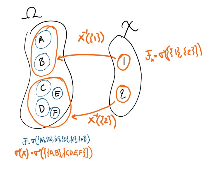
So lets go back to the example! In this case, we find that \(\sigma(Y,Z) = \mathcal F\). We do not lose information about events over the sample space \(\Omega\) if we instead work with events over the joint space \(Y \times Z\). On the other hand, \(\sigma(Y,X) \subset \mathcal F\) - we do get information loss here.

The variable \(Z\) contains better resolution about events than \(X\) do. This is captured by the relation \(\sigma(X) \subset \sigma(Z)\). Whenever we have an ordered chain of \(\sigma\)-algebras \(\mathcal F_0 \subset \mathcal F_1 \subset ... \subset \mathcal F\), we call this a filtration. If we have random elements \(\{X_k\}_k\) so that \(X_k\) is measurable with respect to \(\mathcal F_k := \sigma(X_0,X_1,...X_k)\) for all \(k\) we say the variables are adapted, and we call the filtration natural. In this case, we have a natural filtration \(\sigma(X)\subset\sigma(X,Z)\subset \mathcal F\).

The filtration can be seen though how a genererators for each algebra get 'smaller'. E.g. {C,D,E,F} is a superset of {E,F} is a superset of F.

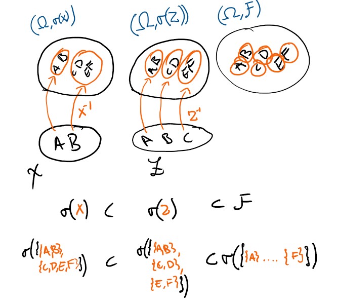
Since every event in \(\sigma(X)\), is in \(\sigma(Z)\), the random element \(X\) is measurable with respect to \(\sigma(Z)\) as well as to \(\mathcal F\). We use the alternative notation \(X \in \sigma(Z)\), and say that \(X\) is measurable with respect to \(Z\), or that the random element is measurable with respect to another random element. We can also see that \(Y \not\in \sigma(X)\) for example.

The probability spaces of the random elements

From the measurable function \(X\), a new measure can be derived on \((\mathcal X,\mathcal F_X)\). For any event \(B \in \mathcal F_X\) we use the inverse image \(X^{-1}(B)\), and since \(X\) is measurable that is guaranteed to be an event - it has a measure \(P(X^{-1}(B))=: X \sharp P (B)\). This is called the pushforward measure since we use \(X\) to push \(P\) forwards from \((\Omega,\mathcal F)\) to \((\mathcal X,\mathcal F_X))\). We also introduce the symbols \(P_X=X \sharp P\), \(P_Y=Y\sharp P\) and \(P_Z=Z\sharp P\). If the domain and base measure is understood from context, we use the term law instead. \(P_X=X\sharp P=\operatorname{law}(X)\) etc…

These functions can be computed to be

event \(A\)	\(P_X(A)\)	\(P_Y(A)\)	\(P_Z(A)\)
\(\{A\}\)	\(4/8\)	\(3/8\)	\(4/8\)
\(\{B\}\)	\(4/8\)	\(5/8\)	\(2/8\)
\(\{C\}\)	n/a	n/a	\(2/8\)

We have now constructed ourself three new probability spaces!

• \[(\mathcal X,\mathcal F_X,P_X) = (\mathbb 2,\mathfrak P(\mathbb 2),X \sharp P)\]
• \[(\mathcal Y,\mathcal F_X,P_Y) = (\mathbb 2,\mathfrak P(\mathbb 2),Y \sharp P)\]
• \[(\mathcal Z,\mathcal F_Z,P_Z) = (\mathbb 3,\mathfrak P(\mathbb 3),Z \sharp P)\]

The pushforawrds measure is defined so that the diagram commutes - we may either map from Omega to 2 and then to some probability, or take the sum of individual probabilities over Omega directly.

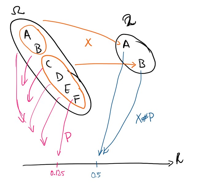
We know that \(X \in \sigma(Z)\). How can we combine that with the new spaces to get more understanding between random elements? For all events \(A_X\in\mathcal F_X\), there exists some event \(A_Z\in\mathcal F_Z\) so that \(X^{-1}(A_X) = Z^{-1}(A_Z)\). We can therefore define a function \(g: (\mathcal Z,\mathcal F_Z) \to (\mathcal X,\mathcal F_X)\) so that \(g \circ Z = X\) and this function is measurable. Considering \(g\) as a function from the probability space \((\mathcal X,\mathcal F_X,P_X)\) we can even call \(g\) a random element over the sample space \(\mathcal Z\).

The filtration allows a factorization. Each pink arrow correspods to some combination of a blue and an orange arrow.

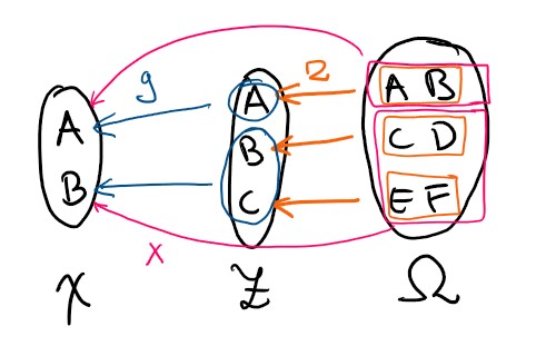
In my example here, the sets are discrete, and the elementary events are included in the \(\sigma\)-algebras, so the function \(g\) is uniquely defined.

1. We extend the function notation in the most sensible way: \(X(A) = \{X(a) : a \in A\}\). ↩

2. Honestly, there seems to be mathematical details here that could lead me astray. My intuition could be wrong - I admit. I have made some checks on finite sets that my intuition holds, so I suspect that there could be cases in infinite spaces that are…. confusing. ↩

3. The symbol \(\times\) denotes the cartesian products of sets. ↩