Benchmarking Quadratic Programming for KMM

What is the best QP solver for kernel mean matching?

I want to solve the QP problem

\[\begin{align*} \min_{w \in \mathbb{R}^n} \frac{1}{2} w^T K w - \kappa^T w \\ 0 \leq w \leq B \\ \left| \sum_{i=1}^n w_i - n \right| = n \epsilon \end{align*}\]

where \(\epsilon\) is some small number, \(B > 0\) is an upper bound, \(K\) is a positive semi-definite matrix, and \(\kappa\) is a vector. The problem arises in kernel mean matching (see Gretton et al. 2008 for more details). The quadratic coefficients are \(K[i,j] = k(x_i, x_j)\), where \(k\) is a kernel function and \(x_i\) are data points from the training dataset. The linear coefficients are given by \(\kappa[i] = n \frac{1}{n_{te}} \sum_{j=1}^{n_{te}} k(x_i, y_j)\) where \(y_j\) are data points from the test dataset of size \(n_{te}\).

I simplify the problem by replacing \(\left| \sum_{i=1}^n w_i - n \right| = n \epsilon\) with \(\sum_{i=1}^n w_i = n\). As they point out in the paper, this should have very little impact if \(n\) is large. Doing this removes a hyperparameter and a variable from the problem. I selected \(B = 100\), quite arbitrarily.

To numerical precision, the matrix \(K\) may not be positive semi-definite (PSD). In my case it has several eigenvalues at zero. Due to numerical imprecision, some turn out small and negative. This is a problem for the solvers, since they require the matrix to be PSD. We must stabilize the problem somehow.

I first tried projection to the PSD cone via eigenvalue pruning. This means we compute the eigenvalue decomposition of \(K\), and set all negative eigenvalues to zero. \(V\) is the matrix of eigenvectors and \(\Lambda\) is the diagonal matrix of eigenvalues. The eigenvalues are sorted so that \(\lambda_1 \geq \lambda_2 \geq \dots \geq \lambda_n\). The expression \((\lambda_i)^+ = \max(0, \lambda_i)\) is the ReLU, i.e. replace by zero if negative.

\[\begin{align*} K = V \Lambda V^T = V \operatorname{diag}( \lambda_1, \dots, \lambda_n ) V^T \\ K^{proj} = V \operatorname{diag}( (\lambda_1)^+, \dots, (\lambda_n)^+ ) V^T \end{align*}\]

Unfortunately, numerical errors sometimes made it so that the resulting matrix still was not positive semi-definite, despite this procedure.

Next attempt was introducing a diagonal shift. I use an RBF kernel for \(k(\cdot, \cdot)\), so \(k[i,i] = 1\) always. The off-diagonal elements \(K[i,j] < 1\) if \(i \neq j\). Adding a small constant to the diagonal should shift the spectrum towards nonnegative values. This is a standard trick in Gaussian process regression, where it corresponds to adding L2 regularization. It seems like a natural thing to try here as well. The exact size of the perturbations of the eigenvalues should be given by the Gershgorin circle theorem (also called the Geršgorin Discs). I did not do the full analysis, but that could be a starting point for anyone who wants to look into this further.

The formula I use is

\[K^{shift} = K + I (e - \lambda_n)\]

where \(I\) is the identity matrix. The most negative eigenvalue is \(\lambda_n\). The offset \(e\) is just for numerical stability. I chose \(e = 10^{-3}\). This seemed to solve my precision issues.

Result from first runs

I set up a handful of solvers on my MacBook Pro M1 (8 cores and 32GB of RAM). I subsample \(m\) data points when constructing the \(K\) and \(\kappa\) matrices, prune the PSD-ness with the shifting method, and run the solvers on progressively larger problems until a single solve takes more than 60 seconds or the problem size exceeds 13,000. The time for shifting eigenvalues is excluded since it is the same for all solvers.

I tried scipy.optimize.minimize, mosek, cvxpy, cvxopt and qpsolvers. All but mosek have a wide variety of solver backends.

From early exploration, I decided to skip

• scipy.optimize.minimize since it is very slow on large problems. It was the only non-dedicated QP solver in this benchmark.
• qpsolvers-highs also slowed down catastrophically on larger problems. I think it is tuned to be good on sparse problems.
• qpsolvers-ecos did not believe my matrix was positive semi-definite, despite my efforts.
• qpsolvers-proxqp since it needed some libc++ version I had not installed on my MacBook.

Skipping these, I tried a couple of backends for each library, and recorded the solve time.

Runtime from first run on my laptop.

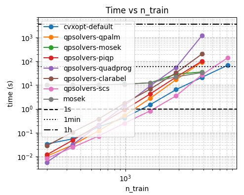
From this, I learn:

• mosek has nicer asymptotics, but higher setup cost.
• scs and cvxopt are quite similar in runtime.
• cvxpy as a frontend failed. It had worked on my toy problem for developing the code, but it failed on the real problem. Maybe it does some preprocessing, maybe I made a mistake. It does seems there are promising backends available to me in the other libraries, so I will just use those instead.

I did check the values of the solutions found, and all solvers were really close. So we can now move on to the next step, which is to try to solve the problem on more data.

Fewer solvers, larger problems

I wanted to look into scs, mosek and cvxopt. The runtime is reported relative to cvxopt.

Runtime from second run on my laptop.

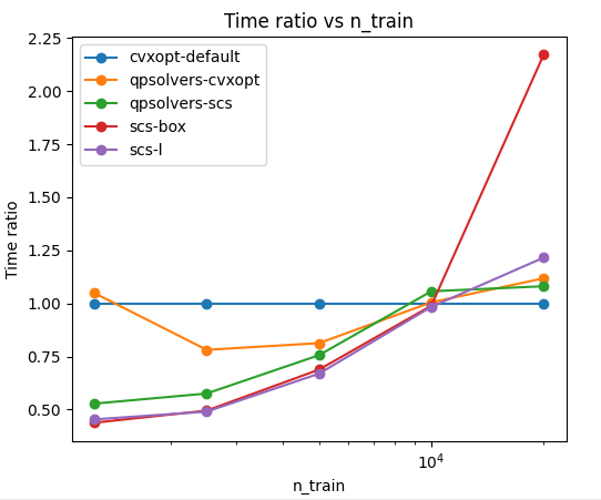
From this, I learn that cvxopt is fastest as the problem scales up. Running it via the qpsolvers frontend had a setup cost of ~10% (about 1 minute).

SCS seemed so promising at smaller sample sizes that I spent the time to learn its API and encode the problem in two different ways. A box constraint like \(0 \leq w \leq B\) can be encoded in two different ways:
(1) Linear cone uses two separate constraints \(-w + s_1 = 0\) and \(w + s_2 = B\), with the slack variables \(s_1, s_2 \geq 0\) lying in the linear cone (scs-l in the plot), or (2) Box cone (scs-box in the plot), meaning we encode the constraint as \(w + s = 0\), with \(-tB \leq s \leq 0\), and add a new constraint \(t = 1\). This reduces the number of slack variables, but we see in the runtime it is much more expensive to compute.

SCS can be compiled with MKL support, which I could use on my compute server. That was a speedup of ~20%. There is also some sort of CUDA support in SCS, but the documentation is a bit lacking, and I did not manage to install it. This might have to be an exploration for another time.

Conclusion

The general learning is that you should try different solvers on your problem. The problem size and structure matter a lot. When you have found a solver that seems right, investigate how it scales. Learnings from one problem size may not be valid for another. If you need to solve the program many times, you should circumvent the frontend and use the optimizer directly. You may shave off some time by skipping the problem setup cost, and you may get access to more advanced features.