Analysing Net Benefit Analysis

This post is an exploration of the “NetBenefit curves” of Vickers and Elkin, also promoted by Steyerberg. I run regressions on some dataset, and investigate both the Net Benefit framework, and also the impact of using a balanced loss vs standard loss (as often done when faces with class imbalance and label shift)

Sneak peek of the conclusions:

A balanced regression has a better balanced accuracy, but worse calibration. The AUROC is comparable. The net benefit is worse (likely due to miscalibration)
The net benefit curve indicates that either predictor can be best, if optimizing the decision threshold \(\tau\) instead of using the default \(\tau=p_t\). Without optimizing for net benefit, the balanced models perform substantially worse.
It seems like the NetBenefit is sensitive to both label and covariate shift. While the balanced accuracy, is invariant to label shift (sometimes called ‘prevalence invariance’)

I assume you are familiar with the ROC and the calibration plot for binary classifiers. In this section, we introduce the net benefit curve of Vickers and Elkin.

Defining the Net Benefit curve

We want to evaluate a diagnostic tool. Either a diagnosis is made \((t=1 \text{ or } t=0)\). Either the disease is present or not \((y=1 \text{ or } y=0)\). The diagnosis is stated based on some observable parameters \(x\). The fact that we make the diagnosis does not affect whether the disease is present or not, so \(T \perp Y \lvert X\).

Diagnostic tools, when used on \(N\) separate patients, give a number of true positives (TP= \(\#\{t=y=1\}\)), false positives (FP= \(\#\{t=1,y=0\}\)), false negatives (FN= \(\#\{t=0,y=1\}\)) and true negatives (TN= \(\#\{t=y=0\}\)). If the utility (e.g. expected number of QUALYs) for each of these cases is a, b, c and d, the utility for our model per patient, will be “benefit” \(B =\frac{1}{N} (a\cdot{}TP+b\cdot{}FP+c\cdot{}FN+d\cdot{}TN)\).

If we never make a diagnosis, \(t=0\) always, and we get find \(B_{none}=\frac{1}{N}(b\cdot{}FN+d\cdot{}TN)\). This can be taken as a reference level, and we can talk about the Net Benefit as the change from this zero-level. It is the case that the number of disease is constant in the population, independant of our diagnosis, so if \(D = \#\{y=1\}\), then \(FN+TP=D\) and \(TN+FP=N-D\). The baseline benefit (no treatment) is thus \(B_{none} = (bD + d(N-D))/N\) This gives a (provisionary) formula for the net benefit \(B - B_{none} = \frac{(a-c)TP + (b-d)FP}{N}\).

We can just as well scale the net benefit by dividing by \((a-c)\) and define \(w=(b-d)/(a-c)\) to simplify the formula:

\[NB=\frac{1}{N}( TP + w\cdot{}FP )\]

If the exact probability that a patient has the disease, \(\rho=p(y=1\lvert{}x)\) was known, the choice choose to make a diagnosis would have expected utility \(a\cdot{}\rho + b\cdot(1-\rho)\). The expected utility of not diagnosing would be \(c\cdot{}\rho{}+d\cdot(1-\rho{})\). The probability \(p_t\) where diagnosing and not diagnosing is of equal utility is the solution to

\[ap_t + b(1-p_t) = cp_t+d(1-p_t)\]

Algebra gives that

\[p_t /(1-p_t) = (b-d)/(a-c) = w\]

so we can parametrize the net benefit function at various threshold probabilitites \(p_t\).

Assume you have a probabilistic model \(f(x) \in [0,1]\). To get a diagnose decision, one must use a cut-point \(\tau\), stating the diagnose if the model outputs a number above the threshold; \(t=1\{f(x) > \tau\}\). By default, \(\tau=0.5\), but one can change the cut-point. Adjusting the cut-point is the key idea of the reciever operating characteristic curve (ROC) for example. Vickers and Elkin dictates you should set \(\tau=p_t\).

Finally, sweep the threshold \(p_t\) and plot the net benefit at each \(p_t\) for you model!

Remarks

The net benefit calculation suffers some problems. The first one is that it is dependant on the feature distribution. Considering the law of large numbers, the net benefit curve is a consistent estimator of

\[p(t=1,y=1) + w\cdot{} p(t=1,y=0) = p(t=1\lvert{}y=1)p(y=1) + w\cdot{} p(t=1\lvert{}y=0)p(y=0)\]

but in case there is distribution shift, this quantity will not generalize from the training data to future test data. Normally, we consider the quantities Sensitivity and Specificiy, since these depend on the conditional quantity

\[p(t\lvert{}y) = \int_{x} p(t|x)p(x|y) \,\mathrm{d}x = \int_{x} 1\{f(x) > \tau\} p(x|y) \,\mathrm{d}x\]

which might bu invariant, despite changes in \(p(y)\) (this is a so called label shift, of a prevalence change). In other words: the net benefit computed on one dataset might not be indicative of the net benefit on another dataset, if there is label shift in the data.

The second issue is the choice of cut-point \(\tau=p_t\), which might not be optimal. For every \(p_t\), there is some \(\tau_{opt}\) that maximizes the net benefit. If the model is perfect, \(f(x) = p(y=1\lvert{}x)\), then it seems that \(\tau_{opt}=p_t\). If the model is not perfect this choice might not be optimal. Remember that if you optimize for \(\tau_{opt}\), do so not over the test data, to avoid data leakage.

Doing the analysis

We make it all in jupyter notebooks. Start with imports.

import numpy as np
import matplotlib.pyplot as plt
import sklearn.datasets
import sklearn.model_selection
import sklearn.linear_model
import sklearn.calibration
import matplotlib.collections 
import sklearn.ensemble
import sklearn.tree

Then define a class to do the Net Benefit analysis. It is spaghetti code, but it works.

class NetBenefit:
    """Make a Net Benefit curve
    
    API similar to sklearn.metrics.RocCurveDisplay.from_predictions and sklearn.calibration.CalibrationDisplay.from_predictions

    The code evolved quite organically and is not very clean. 
    If you want to use it - beware of bugs!
    """
    def __init__(self,ax):
        self.ax = ax

    @staticmethod
    def net_benefit(tp,fp,pt,n):
        """Compute the net benefit equation, but handle edge cases
        
        NB = (TP - w*FP) / N

        """
        w = pt / (1-pt) if pt < 1 else np.inf
        if fp == 0:
            return tp / n
        elif w == np.inf and fp > 0:
            return -np.inf
        else:
            return (tp - w*fp) / n

    @staticmethod
    def optimal_threshold(y_true, p_hat, pt):
        """Find the threshold that maximizes the net benefit
        
        Since the function might be non-convex, we brute force search by gridding
        """
        pts = np.linspace(0,1,200)
        nb = np.zeros(len(pts))
        for i,pt in enumerate(pts):
            yhat = p_hat>pt
            true_positives = (yhat & y_true).sum() 
            false_positives = (yhat & ~y_true).sum()
            nb[i] = NetBenefit.net_benefit(true_positives, false_positives, pt, len(y_true))
        return pts[np.argmax(nb)]

    def add_to_ax(self, name, pts, nb=None, nb_all=None, nb_opt=None):
        """Add net benefit curves to the axes"""

        ax = self.ax
        if 'Policy "None"' not in ax.get_legend_handles_labels()[1]:
            ax.axhline(0, color='k', linestyle='dashed', label='Policy "None"')

        if 'Policy "All"' not in ax.get_legend_handles_labels()[1] and nb_all is not None:
            # https://stackoverflow.com/questions/7386872
            col = matplotlib.collections.LineCollection([np.column_stack((pts,nb_all))], colors='grey',label='Policy "All"')
            ax.add_collection(col, autolim=False)

        if nb is not None:
            ax.plot(pts,nb, label=f'{name} Standard')

        if nb_opt is not None:
            ax.plot(pts,nb_opt, label=f'{name} Optimized', linestyle='dotted')

        ax.set_xlabel('Threshold $$p_t$$')
        ax.set_ylabel('Net benefit')
        ax.legend()

    @classmethod
    def from_predictions(cls,y_test, p_hat, ax, name):
        """Create the NetBenefit curve from predictions"""
        out = cls(ax)

        nb = np.zeros(100)
        nb_opt = np.zeros(len(nb))
        nb_all = np.zeros(len(nb))
        ndata = len(y_test)
        pts = np.linspace(0,1,len(nb))
        for i,pt in enumerate(pts):
            yhat = p_hat>pt
            true_positives = (yhat & y_test).sum() 
            false_positives = (yhat & ~y_test).sum()
            nb[i] = NetBenefit.net_benefit(true_positives, false_positives, pt, len(y_test))

            yhat = np.full(ndata, True)
            true_positives = (yhat & y_test).sum()
            false_positives = (yhat & ~y_test).sum()
            nb_all[i] = NetBenefit.net_benefit(true_positives, false_positives, pt, len(y_test))

        out.add_to_ax(name, pts, nb=nb, nb_all=nb_all)
        return out

    @classmethod
    def from_estimator(cls, estimator, X_test, y_test, ax, name, X_train=None, y_train=None):
        """If X_train and y_train are supplied, the optimal threshold is computed on the training data used in liu of p_t"""
        phats = estimator.predict_proba(X_test)[:,1]

        out = cls.from_predictions(y_test, phats, ax, name)

        if X_train is not None and y_train is not None:
            nb_opt = np.zeros(100)
            pts = np.linspace(0,1,len(nb_opt))
            phat_train = estimator.predict_proba(X_train)[:,1]
            for i,pt in enumerate(pts):
                tau = NetBenefit.optimal_threshold(y_train, phat_train, pt)
                p_hat = estimator.predict_proba(X_test)[:,1]
                yhat = p_hat>tau
                true_positives = (yhat & y_test).sum() 
                false_positives = (yhat & ~y_test).sum()
                nb_opt[i] = NetBenefit.net_benefit(true_positives, false_positives, pt, len(y_test))

            out.add_to_ax(name, pts, nb_opt=nb_opt)

        return out

We analyze the model performance in discrimination (ROC), calibration, and net benefit. The next code block shows how we train the model and produce the relevant plots.

We are also interested in how using a balanced loss function affects the model performance compared to a standard one, so the code runs twice: unbalanced and balanced. This will matter for datasets with class imbalance.

def analyze(X,y,name, model):
    X_train, X_test, y_train, y_test = sklearn.model_selection.train_test_split(X,y,test_size=0.2,random_state=0)

    clf = model
    clf.fit(X_train,y_train)
    fig,axs = plt.subplots(1,3, figsize=(15,5))
    sklearn.metrics.RocCurveDisplay.from_estimator(clf,X_test, y_test,ax=axs[0], name='Unbalanced')
    sklearn.calibration.CalibrationDisplay.from_estimator(clf,X_test, y_test,ax=axs[1],n_bins=10, name='Unbalanced')
    NetBenefit.from_estimator(clf, X_test, y_test, ax=axs[2], name='Unbalanced', X_train=X_train, y_train=y_train)
    y_hat = clf.predict(X_test)
    acc_unbalanced = sklearn.metrics.accuracy_score(y_test, y_hat)
    balacc_unbalanced = sklearn.metrics.balanced_accuracy_score(y_test, y_hat)

    if isinstance(clf, sklearn.ensemble.AdaBoostClassifier):
        clf.estimator.class_weight='balanced'
    else:
        clf.class_weight='balanced'

    clf.fit(X_train,y_train)
    sklearn.metrics.RocCurveDisplay.from_estimator(clf,X_test, y_test,ax=axs[0], name='Balanced')
    sklearn.calibration.CalibrationDisplay.from_estimator(clf,X_test, y_test,ax=axs[1],n_bins=10, name='Balanced')
    NetBenefit.from_estimator(clf,X_test, y_test, ax=axs[2], name='Balanced', X_train=X_train, y_train=y_train)
    y_hat = clf.predict(X_test)
    acc_balanced = sklearn.metrics.accuracy_score(y_test, y_hat)
    balacc_balanced = sklearn.metrics.balanced_accuracy_score(y_test, y_hat)

    s1 = f"{name}. $$n_={len(y_train)}$$, $$n_={len(y_test)}$$ Class balance: (train) {y_train.mean():.2%}, (test) {y_test.mean():.2%}."
    s2 = f"Unbalanced: Acc={acc_unbalanced:.2%}, BalAcc={balacc_unbalanced:.2%}. Balanced: Acc={acc_balanced:.2%}, BalAcc={balacc_balanced:.2%}."
    fig.suptitle(s1 + "\n" + s2)

Create three datasets to analyze:

A diabetes dataset on OpenML originally from UCI.
A synthetic dataset with same number of features and samples, but with a different distribution and more class imbalance.
A larger synthetic dataset with many more samples and features, but some of the features are spurious, potentially providing spurious correlations. Regularization is needed!

X_diabetes,y_diabetes  = sklearn.datasets.fetch_openml(data_id=37,return_X_y=True,as_frame=False)
assert set(y_diabetes) == {'tested_positive','tested_negative'}
y_diabetes = (y_diabetes=='tested_positive').astype(int)

X_synth1,y_synth1 = sklearn.datasets.make_classification(n_samples=768,n_features=8,n_classes=2,weights=[0.80,0.20],random_state=0)
X_synth2,y_synth2 = sklearn.datasets.make_classification(n_samples=10_000,n_features=400, n_informative=20,n_classes=2,weights=[0.95,0.05],random_state=0)

Try a logistic regression with L2 penalty from cross validation! How does it go?

for X,y,name in (
    (X_diabetes,y_diabetes,'Diabetes'),
    (X_synth1,y_synth1,'Synthetic 1'),
    (X_synth2,y_synth2,'Synthetic 2')
 ):
    analyze(X,y,f"LogRegCV on {name} dataset",model = sklearn.linear_model.LogisticRegressionCV(max_iter=1000))

We found:

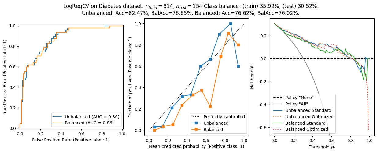
On the real world data, the balanced logistic regression and the unbalanced one are virtually the same in terms of ROC – the class imbalance is clearly not a problem. The calibration is similar between the two models, and the net benefit is also similar.
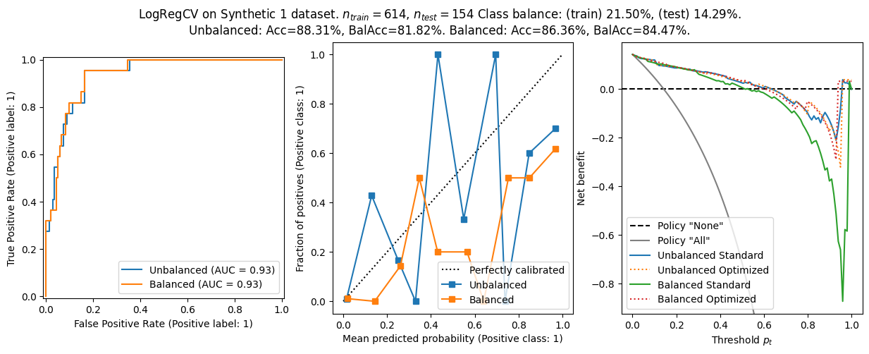
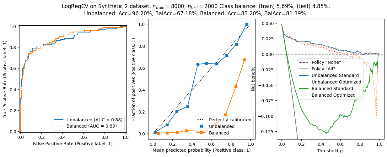
On the synthetic datasets, the balanced logistic regression has a better balanced accuracy, but worse calibration. The AUROC is comparable.
The balanced models shows worse calibration generally. That makes sense since the optimization target is not \(f(x)\approx{}p(y=1\lvert{}x)\).
The net benefit curves are worse for the balanced model on the synthetic datasets. I suspect this is due to miscalibration.
On Synthetic dataset 2, we show that the combination of distribution shift and miscalibration create a bad tradeoff, hurting the net benefit. Using the decision threshold \(\tau_{opt}\) improves the situation considerably.
Optimizing the threshold for net benefit can sometimes, for some \(p_t\), make the balanced model perform better than the unbalanced one.

As a last analysis, I redid the analysis using a AdaBoost classifier. Some experimentation showed this was very sensitive to the selection of hyperparmeters. I have kept some hyperparameters that gave reasonable performance. If continuing this analysis, I would recommend using some automatic hyperparameter optimization to improve performance.

for X,y,name in (
    (X_diabetes,y_diabetes,'Diabetes'),
    (X_synth1,y_synth1,'Synthetic 1'),
    (X_synth2,y_synth2,'Synthetic 2')
 ):
    analyze(X,y,f"AdaBoost on {name} dataset",model = sklearn.ensemble.AdaBoostClassifier(n_estimators=200,learning_rate=0.05,algorithm='SAMME',random_state=0,estimator=sklearn.tree.DecisionTreeClassifier(criterion='log_loss',max_depth=1)))

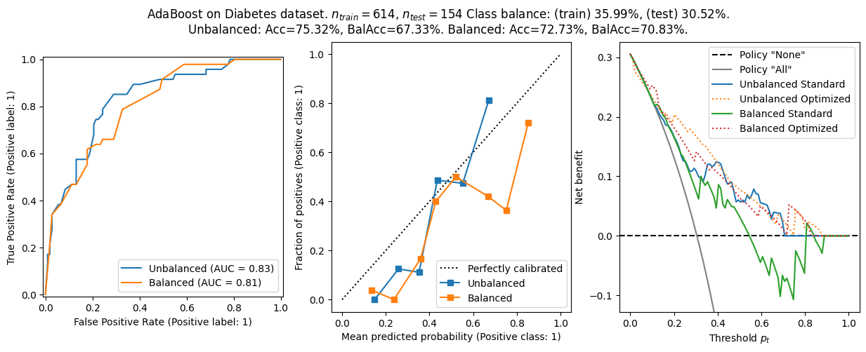
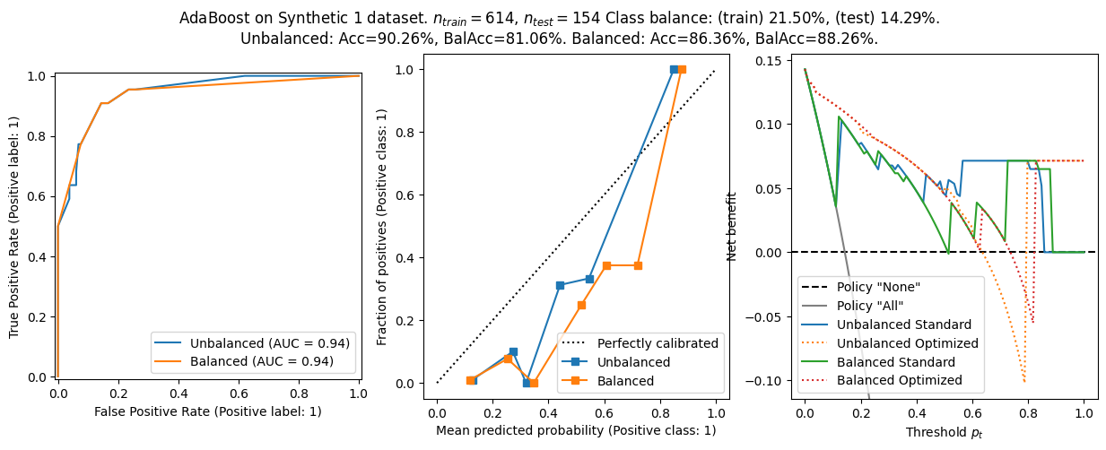
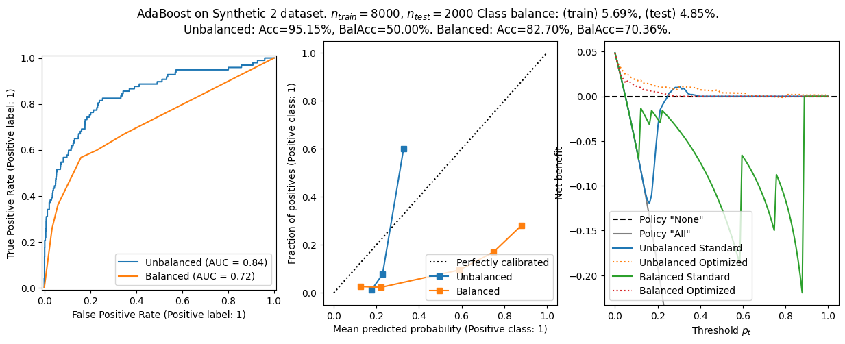
The general conclusion from before still holds:

Balanced models have better balanced accuracy, but worse calibration and worse net benefit.
The choice \(\tau=p_t\) is not optimal in general, and using this heuristic lead to worse net benefit - especially in ill calibrated models.

Ludvig Hult

Defining the Net Benefit curve

Remarks

Doing the analysis