
Variational Inference - An Example Calculation
I was working though problems from the compendium Pattern Recognition - Fundamental Theory and Exercise Problems by Arne Leijon and Gustav Eje Henter. One of the problems on variational inference was interesting and a little complicated. So this post is a walk-though computation for how to solve it. In my version of the compendium (2013, date unspecified) it is called problem 9.4. I formulate it just slightly differently and more open, so that the reasoning shows clearly.
The battle plan is to
- Formulate the problem as a bayesian inference problem
- Come up with a prior on the parameters
- Formulate the likelihood
- Compute the posterior. Realize it is not possible to solve on closed form. Use variational inference and a factor approximation.
- Compute the predictive.
- Run a numerical illustration
But first, some notation. If \(\mathcal{N}(\mu,\sigma^2)\) is a normal distribution, its density is \(\mathcal{N}(x;\mu,\sigma^2)\). Similarly for Bernoulli variables \(\text{Ber}(p)\) and beta variables \(\text{Beta}(a,b)\). Both probability mass functions and density functions are denoted \(f_X(x)\), with the random variable (\(X\)) and the concrete value (\(x\)) written out.
We will also work a lot with gaussians. They have a convolution rule
\[\int \mathcal{N}(x;\mu_1,\sigma_1^2)\mathcal{N}(x;\mu_2, \sigma_2^2) \,\text{d}x = \mathcal{N}(\mu_1;\mu_2,\sigma_1^2+\sigma_2^2)= \mathcal{N}(\mu_2;\mu_1,\sigma_1^2+\sigma_2^2)\]They have rules for swapping, flipping, and scaling
\[\mathcal{N}(x;y,s^2) = \mathcal{N}(y;x,s^2)\] \[\mathcal{N}(x;0,s^2) = \mathcal{N}(-x;0,s^2)\] \[\mathcal{N}(ma;x,s^2)= \mathcal{N}(a;x/m,s^2/m^2)\]Problem statement
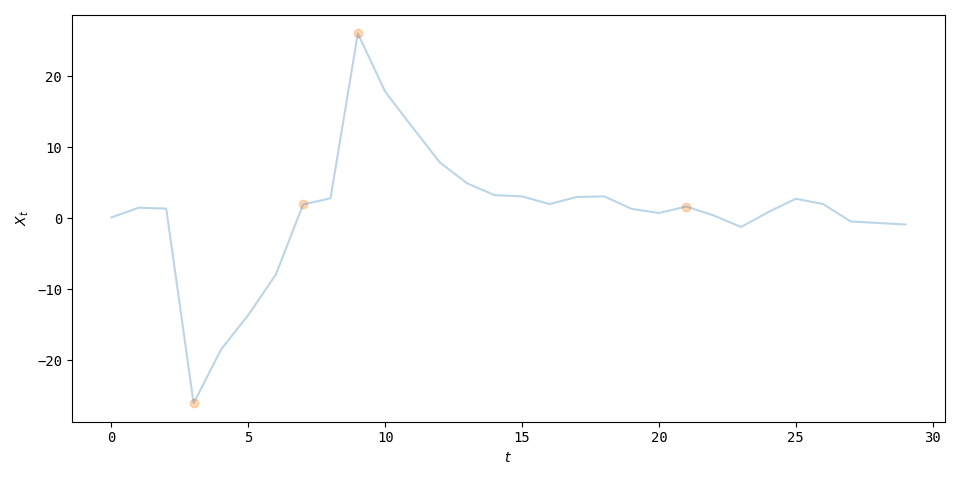
You have a data generator
\[X_0 = 0\] \[X_t = aX_{t-1}+cU_t+dZ_tV_t \quad t=1,\dots{},T\]The data \(X_t\) is observed for all \(t=1,\dots{},T\). The parameters \(d,c\) are constant and assumed known. The variables \(U_t,V_t \sim \mathcal{N}(0,1)\) are standard normal and independent. The variables \(Z_t \sim \text{Ber}(w)\) are independent 0-1 distributed variables.
Define the observed data vector \(\underline{x} = (x_1,x_2,...x_T)\) and the unobserved noise vector \(\underline{z}=(z_1,z_2,...z_T)\).
Make a bayesian inference about the parameters \(w\) and \(a\). What is the mean parameter estimates? The credibility intervals? What is predictive distribution? Its mean and variance?
Interpretation
Consider a truck that drives on a gravel road. It rocks back and forth, and if the rocking is not too bad, we can model the leaning angle at time \(t\) as a random variable \(X_t\). The truck has overdamped suspension so the leaning angle returns to 0 in a rate proportional to the current angle. So ideally, \(X_t = aX_{t-1}\) with \(a \in (0,1)\).
However, there are many small bumps in the gravel. The road is equally bumpy everywhere, and there are so many small bumps that the average bump under time \(t\) is well described by a normal distribution (consider central limit theorem). This is modelled by a white noise process, which we call \(cU_t\).
There are also big bumps in the road. They are much rarer, and we think at worst a single big bump can happen for each time step \(t\). If there is a big bump at time \(t\) (indicated by \(Z_t=1\)), the effect of the bump is modelled by a gaussian displacement, but with large standard deviation \(d\). This is a Bernoulli process multiplied by a Gaussian process, and we denote it \(dZ_tV_t\).
The prior
The first step for bayesian inference is to select priors. Since \(w\) is a probability, the prior should have support covering \([0,1]\). A standard choice is \(W\sim \text{Beta}(\alpha_0,\beta_0)\). How do we select \(\alpha_0,\beta_0\)? Lets take the Jeffreys prior, i.e. \(f_W(w) \propto \sqrt{I(w)}\) the prior density must be proportional to the square root of the fisher information.
\[\begin{aligned} \ln f_{Z_t\mid{}W}(z\mid{}w) =& z_t\ln w +(1-z_t)\ln (1-w)\\ I(w) =& \mathbb E\left[ \left(\frac{\partial}{\partial z_t} \ln f_{Z_t\mid{}W}(z\mid{}w) \right)^2 \mid w \right] \\ =& \mathbb E\left[ \left( \frac{z_t}{w} - \frac{1-z_t}{1-w} \right)^2 \mid w \right] \\ =& w\left( \frac{1}{w} - \frac{0}{1-w} \right)^2 + (1-w)\left( \frac{0}{w} - \frac{1}{1-w} \right)^2 \\ =& \frac{1}{w(1-w)} \end{aligned}\]Choose \(f_W(w) \propto \sqrt{ \frac{1}{w(1-w)}} = w^{\frac{1}{2}-1}(1-w)^{\frac{1}{2}-1}\), or in other words, \(\alpha_0=\beta_0=\frac{1}{2}\)
Next choose prior for \(a\). We know that \((X_t\vert{}Z_{t-1},Z_t)\) comes from a linear model with gaussian additive noise, and we want to make inference on the slope coefficient. In that setting, gaussian priors are known to be conjugate. Therefore, assume a gaussian prior distributions for \(a\). Pick \(A \sim \mathcal{N}(0,\sigma_0^2)\), and we may choose some large \(\sigma_0^2\), making the prior weakly informative.
The Likelihood
With these priors, we can formulate the likelihood
\[f_{\underline{X},\underline{Z},W,A}(\underline{x}, \underline{z},w,a) = f_{\underline{X}\mid\underline{Z},A}(\underline{x}\mid \underline{z},a) f_{\underline{Z} \mid W}(\underline{z}\mid w) f_{A}(a) f_{W}(w)\]There are four factors, and the for three of them, we already have a closed for expression (they are Bernoulli, Beta and Normally distributed). So lets compute the expression for the first density as well! I will liberally apply the gaussian rules for swapping and scaling and the convolution rule.
\[\begin{aligned} f_{\underline{X}\mid\underline{Z},A}(\underline{x}\mid \underline{z},a) =& \prod_{t=1}^{T} \int f_{X_{t}\mid X_{t-1},A,Z_{t},V_t}(x_t \mid x_{t-1},a,z_t,v_t) f_{V_t}(v_t) \text{d} v_t \\ =& \prod_{t=1}^{T} \int \mathcal{N}(x_t,ax_{t-1}-dz_tv_t,c^2)\mathcal{N}(v_t,0,1) \text{d} v_t \\ =& \prod_{t=1}^{T} \int \mathcal{N}(dz_tv_t,x_t-ax_{t-1},c^2)\mathcal{N}(v_t,0,1) \text{d} v_t \end{aligned}\]If \(z_t=1\) then
\[\begin{aligned} \int \mathcal{N}(dz_tv_t,x_t-ax_{t-1},c^2)\mathcal{N}(v_t,0,1) \text{d} v_t =& \int \mathcal{N}(v_t,\frac{x_t-ax_{t-1}}{dz_t},\frac{c^2}{d^2z_t})\mathcal{N}(v_t,0,1) \text{d} v_t \\ =& \mathcal{N}(0,\frac{x_t-ax_{t-1}}{dz_t},\frac{c^2}{d^2z_t}+1) \\ =& \mathcal{N}(x_t,ax_{t-1},c^2+d^2z_t) \end{aligned}\]If \(z_t=0\) then
\[\begin{aligned} \int \mathcal{N}(dz_tv_t,x_t-ax_{t-1},c^2)\mathcal{N}(v_t,0,1) \text{d} v_t =& \int \mathcal{N}(0,x_t-ax_{t-1},c^2)\mathcal{N}(v_t,0,1) \text{d} v_t \\ =& \mathcal{N}(0,x_t-ax_{t-1},c^2)\\ =& \mathcal{N}(x_t,ax_{t-1},c^2+d^2z_t) \end{aligned}\]So combining both cases
\[\begin{aligned} f_{\underline{X}\mid\underline{Z},A}(\underline{x}\mid \underline{z},a) =& \prod_{t=1}^{T} \mathcal{N}(x_t,ax_{t-1},c^2+d^2z_t) \end{aligned}\]With this in our arsenal, we can compute the log likelihood of data and parameters.
\[\begin{aligned} \ln f_{\underline{X},\underline{Z},W,A}(\underline{x}, \underline{z},w,a) =& \sum_{t=1}^T \left( -\frac{(x_t-ax_t)^2}{2(c^2+d^2z_t) } -\frac{1}{2}\ln (c^2+z_td^2) \right)\\ &+\sum_{t=1}^T \left( z_t\ln w + (1-z_t)\ln (1-w) \right)\\ &-\frac{1}{2\sigma_0^2}a^2 \\ &+ (\alpha_0-1)\ln w + (\beta_0-1)\ln (1-w)+\text{const.} \end{aligned}\]The posterior
In principle, we should now just compute the posterior via bayes rule
\[f_{W,A \mid \underline{X} }(w,a \mid \underline{x}) = \frac{ E[f_{\underline{x},\underline{Z},W,A}(\underline{x}, \underline{Z},w,a)]}{ E[f_{\underline{X},\underline{Z},W,A}(\underline{x}, \underline{Z},W,A)] }\]but the expectation in the denominator is difficult. The standard trick in Bayesian Inference is to ignore the denominator, just compute the numerator and identify it as a known distribution, and then look up the denominator in a table. That won’t work here. So we have to resort to approximations!
Variational inference
We are looking for a function \(q(a,w,\underline{z}) \approx f_{W,A, \underline{Z} \mid \underline{X} }(w,a, \underline{z} \mid \underline{x})\), and hopefully we can marginalize out the \(\underline{z}\)-factor in the end. How do we choose \(q\)? One can show that
\[\operatorname*{arg\,max}_{q} \mathbb E_{q}\left[ \ln \left\{ \frac{ f_{\underline{X},\underline{Z},W,A}(\underline{X}, \underline{Z},W,A) }{q(A,W,\underline{Z})} \right\} \right] = \operatorname*{arg\,min}_{q} D_{KL}(q \Vert f_{W,A, \underline{Z} \mid \underline{X} })\]On the right hand side, we have a KL divergence between our approximation \(q\) and the target log density. And the KL divergence guarantee the existence of a global extremum for when \(q = f_{W,A, \underline{Z} \mid \underline{X}}\). The left hand side is called the ELBO. Since the right hand side is not computable, we try to maximize the ELBO, to get the best approximation possible.
Factor approximation
Make the choice \(q(A,W,\underline{Z})=q_1(A,W)q_2(\underline{Z})\). There is a theorem that proves that
\[\ln q_1(a,w) = \mathbb E_{q_2} [ \ln f_{\underline{X},\underline{Z},W,A}(\underline{x}, \underline{Z},w,a) ] + \text{const.}\]if and only if
\[q_1 = \operatorname*{arg\,max}_{q_1} \mathbb E_{q_1q_2}\left[ \frac{\ln f_{\underline{X},\underline{Z},W,A}(\underline{X}, \underline{Z},W,A)}{q_1(A,W)q_2(\underline{Z})} \right]\]And similarly,
\[\ln q_2(\underline{z}) = \mathbb E_{q_1} [ \ln f_{\underline{X},\underline{Z},W,A}(\underline{x}, \underline{z},W,A) ] + \text{const.}\]if and only if
\[q_2 = \operatorname*{arg\,max}_{q_2} \mathbb E_{q_1q_2}\left[ \frac{\ln f_{\underline{X},\underline{Z},W,A}(\underline{X}, \underline{Z},W,A)}{q_1(A,W)q_2(\underline{Z})} \right]\]So we can take turns computing \(q_1\) and \(q_2\), always improving our ELBO. And this is guaranteed to converge to a local maximum. So lets do that computation!
Actual computation
Solving \(q_1\)
\[\begin{aligned} \ln q_1(a,w) =& \mathbb E_{q_2} [ \ln f_{\underline{X},\underline{Z},W,A}(\underline{x}, \underline{Z},w,a) ] + \text{const.} \\ =& \sum_{t=1}^T \mathbb E_{q_2} \left[ -\frac{(x_t-ax_t)^2}{2(c^2+d^2z_t) } \right]\\ &+\sum_{t=1}^T \left( \mathbb E_{q_2}[z_t]\ln w + (1-\mathbb E_{q_2}[z_t])\ln (1-w) \right)\\ &-\frac{1}{2\sigma_0^2}a^2 \\ &+ (\alpha_0-1)\ln w + (\beta_0-1)\ln (1-w)\\ &+\text{const.} \\ =& (\alpha_0 + \sum_{t=1}^{T}E_{q_2}[Z_t] -1)\ln w + (\beta_0+\sum_{t=1}^{T}\mathbb{E}_{q_2}[1-Z_t] -1)\ln (1-w) \\ &-\frac{1}{2} \frac{a^2}{\sigma_0^2}- \frac{1}{2} \sum_{t=1}^T \mathbb E_{q_2} \left[ -\frac{(x_t-ax_t)^2}{(c^2+d^2z_t) } \right] \end{aligned}\]At this stage, we see that the terms for \(w\) and the terms for \(a\) are independent, so the natural factorization \(q_1(a,w) = q_{1A}(a)q_{1W}(w)\) falls out. Introduce \(\gamma_t = E_{q_2}[z_t]\), and see that
\[\ln q_{1W}(w) = (\alpha_0 + \sum_{t=1}^{T}\gamma_t -1)\ln w + (\beta_0+\sum_{t=1}^{T}(1-\gamma_t) -1)\ln (1-w) + \text{const.}\]This density can be identified as a Beta! Define \(\alpha_T = \alpha_0 + \sum_{t=1}^{T}\gamma_t\) and \(\beta_T = \beta_0+\sum_{t=1}^{T}(1-\gamma_t)\). Obtain
\[q_{1W}(w) = \text{Beta}(w ; \alpha_T, \beta_T)\]The terms for \(a\) needs a bit of massage. First state
\[\ln q_{1A}(a) = -\frac{1}{2} \frac{a^2}{\sigma_0^2}- \frac{1}{2} \sum_{t=1}^T \mathbb E_{q_2} \left[ \frac{(x_t-ax_t)^2}{(c^2+d^2z_t) } \right] + \text{const.}\]Next, because of a markov condition \(Z_t\) is independent from \(Z_{t'}\), when conditioned on \(X_t\). Since \(q\) models a conditioned-on-\(\underline{X}\)-distribution, have that \(q_2(\underline{z}) = q_{21}(z_1)q_{22}(z_2)\cdots q_{1T}(z_T)\). This allows the evaluation of the expectation
\[\mathbb E_{q_2} \left[ \frac{(x_t-ax_t)^2}{(c^2+d^2z_t) } \right] = \gamma_t \frac{(x_t-ax_t)^2}{(c^2+d^2) } + (1-\gamma_t) \frac{(x_t-ax_t)^2}{c^2 }\]Inserting this back, expanding all squares, yields
\[\ln q_{1A}(a) = -\frac{1}{2} \frac{a^2}{\sigma_0^2} -\frac{1}{2} \sum_{t=1}^T\gamma_t \frac{a^2x_t^2-2ax_tx_{t-1}}{(c^2+d^2) } -\frac{1}{2} (1-\gamma_t) \frac{a^2x_t^2-2ax_tx_{t-1}}{c^2 } + \text{const.}\]Collecting terms
\[\ln q_{1A}(a) = -\frac{1}{2} \left[ a^2 \left(1+ \sum_{t=1}^T\frac{\gamma_t x_t^2}{c^2+d^2} + \frac{(\frac{1}{\sigma_0^2}-\gamma_t)x_t^2}{c^2} \right) -2a \left( \sum_{t=1}^T\frac{\gamma_t x_tx_{t-1}}{c^2+d^2} + \frac{(1-\gamma_t)x_tx_{t-1}}{c^2} \right) \right] + \text{const.}\]Introduce new notation \(\eta_t = \frac{\gamma_t }{c^2+d^2} + \frac{(1-\gamma_t)}{c^2}\)
\[\ln q_{1A}(a) = -\frac{1}{2} \left[ a^2 \left(\frac{1}{\sigma_0^2}+ \sum_{t=1}^T\eta_t x_t^2 \right) -2a \left( \sum_{t=1}^T \eta_t x_tx_{t-1} \right) \right] + \text{const.}\]More notation \(\sigma_T^2 = \frac{1}{\frac{1}{\sigma_0^2}+ \sum_{t=1}^T\eta_t x_t^2}\) giving
\[\ln q_{1A}(a) = -\frac{1}{2} \left[ \frac{a^2 - 2a \left( \sum_{t=1}^T \eta_t x_tx_{t-1} \right) \sigma_T^2 }{\sigma_T^2} \right]+ \text{const.}\]so with \(\mu_T = \sigma_T^2 \sum_{t=1}^T \eta_t x_tx_{t-1} = \frac{\sum_{t=1}^T \eta_t x_tx_{t-1} }{\frac{1}{\sigma_0^2}+ \sum_{t=1}^T\eta_t x_t^2}\) we identify a gaussian distribution
\[q_{1A}(a) = \mathcal{N}(a, \mu_T, \sigma_T^2)\]Solving \(q_2\)
As noted before, \(q_2\) factorizes nicely. Lets look at a factor \(q_{2t}\).
\[\ln q_2(\underline{z}) = \mathbb E_{q_{1A}q_{1W}} [ \ln f_{\underline{X},\underline{Z},W,A}(\underline{x}, \underline{z},W,A) ] + \text{const.}\] \[\begin{aligned} \ln q_{2t}(z_t) =& \mathbb E_{q_{1A}q_{1W}q_{21}q_{22}\cdots{}q_{2(t-1)}q_{2(t+1)\cdots{}q_{2T}}} [ \ln f_{\underline{X},\underline{Z},W,A}(\underline{x}, \underline{z},W,A) ] + \text{const.} \\ =& -\frac{1}{2}\frac{\mathbb{E}_{q_{1A}}(x_t-x_{t-1}A)^2}{c^2d^2z_t} - \frac{1}{2}\ln (c^2+d^2z_t) \\ &+z_t\mathbb{E}_{q_{1W}}[\ln W]+(1-z_t)\mathbb{E}_{q_{1W}}[\ln (1-W)]\\&+ \text{const.} \end{aligned}\]We apply a few tricks now. If \(p \sim \text{Beta}(a,b)\), then \((1-p) \sim \text{Beta}(b,a)\). Also \(\mathbb{E}[p]=\psi(a)-\psi(a+b)\), where \(\psi\) is the digamma function.
\[\begin{aligned} \ln q_{2t}(z_t) =& -\frac{1}{2}\frac{\mathbb{E}_{q_{1A}}[(x_t-x_{t-1}A)^2]}{c^2d^2z_t} - \frac{1}{2}\ln (c^2+d^2z_t) \\ &+z_t\psi(\alpha_T) +(1-z_t)\psi(\beta_T)\\& + \text{const.} \end{aligned}\]Now expand the square in the expectation for \(A\), and use that \(\mathbb{E}_{q_{1A}}[A] = \mu_T\) and \(\mathbb{E}_{q_{1A}}[A^2] = \mu_T^2+\sigma_T^2\), since it is gaussian.
\[\begin{aligned} \ln q_{2t}(z_t) =& -\frac{1}{2}\frac{( \mu_T^2+\sigma_T^2)x_{t-1}^2 - 2\mu_Tx_{t}x_{t-1} + x_{t}^2}{c^2d^2z_t} - \frac{1}{2}\ln (c^2+d^2z_t) \\ &+z_t\psi(\alpha_T) +(1-z_t)\psi(\beta_T)\\& + \text{const.} \end{aligned}\]By omitting the constants, we get un-normalized log-probabilities. To get the regular probabilities for \(Z_t=i\), we drop the constant, set \(z_t=i\). Call the result \(r_{it}\). Exponentiate and normalize!
\[r_{1t} = \psi(\alpha_T) - \frac{1}{2}\ln (c^2+d^2) - \frac{1}{2}\frac{( \mu_T^2+\sigma_T^2)x_{t-1}^2 - 2\mu_Tx_{t}x_{t-1} + x_{t}^2}{c^2+d^2}\] \[r_{0t} = \psi(\beta_T) - \frac{1}{2}\ln (c^2) - \frac{1}{2}\frac{( \mu_T^2+\sigma_T^2)x_{t-1}^2 - 2\mu_Tx_{t}x_{t-1} + x_{t}^2}{c^2}\] \[q_{2t}(z_t) = \frac{\exp[ r_{z_{t}t}]}{ \exp[ r_{0t}]+\exp[ r_{1t}]}\]For Bernoulli variables the mean is the probability of 1, so we can compute
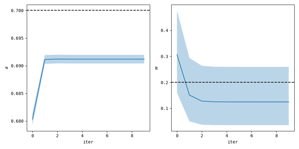
\[\gamma_t = q_{2t}(1) = \frac{\exp[ r_{1t}]}{ \exp[ r_{0t}]+\exp[ r_{1t}]}\]which is needed in our iterative update of parameters. To compute the approximate posterior, we iterate the update equations for \(\gamma_t, \mu_T, \sigma_T\) until the values converge.
When they have converged, \(q_1\) is the posterior on \(a\) and \(w\) that we were seeking.
I have generated some toy data and implemented the estimation procedure. The plots show the data itself and the parameter estimates.
The predictive
The predictive distribution is the distribution of the variable \((X_{T+1}|\underline{X})\). We can use the conditional independencies in the distribution, and construct this conditional as an expectation.
\[f_{X_{T+1}\mid{}\underline{X}}(x_{T+1}\mid{} \underline{x} ) = \int\int\sum_{z_{T+1}=0}^1 f_{X_{T+1}\mid{} A,Z_{T+1},X_{T}}(x_t\mid{}a,z, \underline{x}) f_{Z_{T+1}|W}(z_{T+1}\mid{}w) f_{W|\underline{X}}(w|\underline{x}) f_{A|\underline{X}}(a|\underline{x}) \,\text{d}a\text{d}w\]We have the approximate posterior distributions, and if we plug them in, we get
\[f_{X_{T+1}\mid{}\underline{X}}(x_{T+1}\mid{} \underline{x} ) = \int\int\sum_{z_{T+1}=0}^1 \mathcal{N}(x_{T+1};ax_T,c^2+d^2z_t) \text{Ber}(z_t;w) \text{Beta}(w;\alpha_T,\beta_T) \mathcal{N}(a;\mu_T,\sigma_T^2) \,\text{d}a\text{d}w\]First perform the sum in \(z_t\)
\[f_{X_{T+1}\mid{}\underline{X}}(x_{T+1}\mid{} \underline{x} ) = \int\int \left( w\mathcal{N}(x_{T+1};ax_T,c^2+d^2) + (1-w) \mathcal{N}(x_{T+1};ax_T,c^2)\right) \text{Beta}(w;\alpha_T,\beta_T) \mathcal{N}(a;\mu_T,\sigma_T^2) \,\text{d}a\text{d}w\]Next take the integral over \(w\), and look up beta-expectations in a book.
\[f_{X_{T+1}\mid{}\underline{X}}(x_{T+1}\mid{} \underline{x} ) = \frac{1}{\alpha_T+\beta_T} \int \left( \alpha_T\mathcal{N}(x_{T+1};ax_T,c^2+d^2) + \beta_T\mathcal{N}(x_{T+1};ax_T,c^2)\right) \mathcal{N}(a;\mu_T,\sigma_T^2) \,\text{d}a\]Use the scaling and swapping relations for gaussians and distribute the integral.
\[\begin{aligned} f_{X_{T+1}\mid{}\underline{X}}(x_{T+1}\mid{} \underline{x} ) = &\frac{\alpha_T}{\alpha_T+\beta_T} \int \mathcal{N}(a;\mu_T,\sigma_T^2)\mathcal{N}(a;\frac{x_{T+1}}{x_{T}},\frac{c^2+d^2}{x_T^2} ) \,\text{d}a \\ +&\frac{\beta_T}{\alpha_T+\beta_T} \int \mathcal{N}(a;\mu_T,\sigma_T^2)\mathcal{N}(a;\frac{x_{T+1}}{x_{T}}, \frac{c^2}{x_T^2} ) \,\text{d}a \end{aligned}\]Use the gaussian convolution rule
\[\begin{aligned} f_{X_{T+1}\mid{}\underline{X}}(x_{T+1}\mid{} \underline{x} ) = &\frac{\alpha_T}{\alpha_T+\beta_T} \mathcal{N}(\mu_T;\frac{x_{T+1}}{x_{T}},\frac{c^2+d^2}{x_T^2} +\sigma_T^2) \\ +&\frac{\beta_T}{\alpha_T+\beta_T} \mathcal{N}(\mu_T;\frac{x_{T+1}}{x_{T}},\frac{c^2}{x_T^2} +\sigma_T^2) \end{aligned}\]reuse the scaling property of gaussian densities to reveal that the predictive density is a gaussian mixture
\[\begin{aligned} f_{X_{T+1}\mid{}\underline{X}}(x_{T+1}\mid{} \underline{x} ) = &\frac{\alpha_T}{\alpha_T+\beta_T} \mathcal{N}(x_{T+1};x_T\mu_T,c^2+d^2 +x_T^2\sigma_T^2) \\ +&\frac{\beta_T}{\alpha_T+\beta_T} \mathcal{N}(x_{T+1};x_T\mu_T,c^2 +x_T^2\sigma_T^2) \end{aligned}\]We cannot come any further in this simplification. It is notable that the mean of both components is the same, so \(\mathbb{E}[X_{T+1}\mid{}\underline{x}]=x_T\mu_T\). Variances are also simple in mixture models, and \(\mathbb{V}[X_{T+1}\mid{}\underline{x}] = c^2 +x_T^2\sigma_T^2 + \frac{\alpha_T}{\alpha_T+\beta_T}d^2\).